Tensorflow

2018-10-29 | 阅读：次

一、参数介绍

1. 1 epoch，batch size，iteration

梯度下降法是迭代的，也就是说我们需要多次计算结果，最终求得最优解。梯度下降的迭代质量有助于使输出结果尽可能拟合训练数据。在训练模型时，如果训练数据过多，无法一次性将所有数据送入计算，那么我们就会遇到epoch，batchsize，iterations这些概念。为了克服数据量多的问题，我们会选择将数据分成几个部分，即batch，进行训练，从而使得每个批次的数据量是可以负载的。将这些batch的数据逐一送入计算训练，更新神经网络的权值，使得网络收敛。

Epoch

一个epoch指代所有的数据送入网络中完成一次前向计算及反向传播的过程。由于一个epoch常常太大，计算机无法负荷，我们会将它分成几个较小的batches。

在训练时，将所有数据迭代训练一次是不够的，需要反复多次才能拟合收敛。在实际训练时，我们将所有数据分成几个batch，每次送入一部分数据，梯度下降本身就是一个迭代过程，所以单个epoch更新权重是不够的。
Batch Size

所谓Batch就是每次送入网络中训练的一部分数据，而Batch Size就是每个batch中训练样本的数量.
Iterations

所谓iterations就是完成一次epoch所需的batch个数。batch numbers就是iterations。

简单一句话说就是，我们有2000个数据，分成4个batch，那么batch size就是500。运行所有的数据进行训练，完成1个epoch，需要进行4次iterations。

1.2 Tensor

TensorFlow中数据的中心单元是张量。张量由一组原始值组成，这些原始值被组织成形状为任意维度的数组。张量的秩是其维数。以下是一些张量的例子：

# 一个秩为0的张量；这是一个形状为[]的标量
[1., 2., 3.] # 一个秩为1的张量；这是一个形状为[3]的向量
[[1., 2., 3.], [4., 5., 6.]] # 一个秩为2的张量；这是一个形状为[2, 3]的矩阵
[[[1., 2., 3.]], [[7., 8., 9.]]] # 一个秩为3、形状为[2, 1, 3]的张量

1.3 计算图

TensorFlow 图（也称为计算图或数据流图）是一种图数据结构。很多 TensorFlow 程序由单个图构成，但是 TensorFlow 程序可以选择创建多个图。图的节点是指令；图的边是张量。张量流经图，在每个节点由一个指令操控。一个指令的输出张量通常会变成后续指令的输入张量。TensorFlow 会实现延迟执行模型，意味着系统仅会根据相关节点的需求在需要时计算节点。

张量可以作为常量或变量存储在图中。您可能已经猜到，常量存储的是值不会发生更改的张量，而变量存储的是值会发生更改的张量。不过，您可能没有猜到的是，常量和变量都只是图中的一种指令。常量是始终会返回同一张量值的指令。变量是会返回分配给它的任何张量的指令。

排列成节点的一系列Tensorflow操作。

每个节点将零个或多个张量作为输入，并生成张量作为输出。

构建计算图
运行计算图

node1 = tf.constant(3.0, dtype=tf.float32)
node2 = tf.constant(4.0) # 隐式地表示同样是tf.float32
print(node1, node2)
=====
Tensor("Const:0", shape=(), dtype=float32) Tensor("Const_1:0", shape=(), dtype=float32)

为了在Python中进行有效的数值计算，我们通常使用像NumPy这样的库，这些库执行昂贵的操作，例如Python之外的矩阵乘法，使用以另一种语言实现的高效代码。不幸的是，每次操作都会返回Python，但仍然会有很多开销。如果您想要在GPU上运行计算或以分布式方式运行计算，则这种开销尤其糟糕，因为在这种情况下，传输数据的成本很高。

TensorFlow也在Python之外进行繁重的工作，但为了避免这种开销，它需要更进一步。 TensorFlow不是只独立于Python运行一个单一的昂贵操作，而是让我们描述完全一个完全在Python之外运行的交互操作的图。这种方法类似于Theano或Torch中使用的方法。

因此，Python代码的作用是构建这个外部计算图，并指定应该运行计算图的哪些部分。有关详细信息，请参阅TensorFlow 入门中的计算图部分。

1.3 占位符

我们通过为输入图像和目标输出类别创建节点，来开始构建计算图。

x = tf.placeholder("float", shape=[None, 784])
y_ = tf.placeholder("float", shape=[None, 10])

这里的x和y并不是特定的值，相反，他们都只是一个占位符，可以在TensorFlow运行某一计算时根据该占位符输入具体的值。

输入图片x是一个2维的浮点数张量。这里，分配给它的shape为[None, 784]，其中784是一张展平的MNIST图片的维度。None表示其值大小不定，在这里作为第一个维度值，用以指代batch的大小，意即x的数量不定。输出类别值y_也是一个2维张量，其中每一行为一个10维的one-hot向量,用于代表对应某一MNIST图片的类别。

虽然placeholder的shape参数是可选的，但有了它，TensorFlow能够自动捕捉因数据维度不一致导致的错误。

1.4 变量

为模型定义权重W和偏置b。可以将它们当作额外的输入量，但是TensorFlow有一个更好的处理方式：变量。一个变量代表着TensorFlow计算图中的一个值，能够在计算过程中使用，甚至进行修改。在机器学习的应用过程中，模型参数一般用Variable来表示。

W = tf.Variable(tf.zeros([784,10]))
b = tf.Variable(tf.zeros([10]))

我们在调用tf.Variable的时候传入初始值。在这个例子里，我们把W和b都初始化为零向量。W是一个784x10的矩阵（因为我们有784个特征和10个输出值）。b是一个10维的向量（因为我们有10个分类）。

变量需要通过seesion初始化后，才能在session中使用。这一初始化步骤为，为初始值指定具体值（本例当中是全为零），并将其分配给每个变量,可以一次性为所有变量完成此操作。

sess.run(tf.initialize_all_variables())

1.5 类别预测与损失函数

现在我们可以实现我们的回归模型了。这只需要一行！我们把向量化后的图片x和权重矩阵W相乘，加上偏置b，然后计算每个分类的softmax概率值。

y = tf.nn.softmax(tf.matmul(x,W) + b)

可以很容易的为训练过程指定最小化误差用的损失函数，我们的损失函数是目标类别和预测类别之间的交叉熵。

cross_entropy = -tf.reduce_sum(y_*tf.log(y))

注意，tf.reduce_sum把minibatch里的每张图片的交叉熵值都加起来了。我们计算的交叉熵是指整个minibatch的。

1.6 训练模型

已经定义好模型和训练用的损失函数
tensorflow进行训练
tensorflow知道整个计算图，可以使用自动微分法找到对于各个变量的损失的梯度值
使用最速下降法，步长为0.01

train_step = tf.train.GradientDescentOptimizer(0.01).minimize(cross_entropy)

这一行代码实际上是用来往计算图上添加一个新操作，其中包括计算梯度，计算每个参数的步长变化，并且计算出新的参数值。

返回的train_step操作对象，在运行时会使用梯度下降来更新参数。因此，整个模型的训练可以通过反复地运行train_step来完成。

for i in range(1000):
  batch = mnist.train.next_batch(50)
  train_step.run(feed_dict={x: batch[0], y_: batch[1]})

每一步迭代，我们都会加载50个训练样本，然后执行一次train_step，并通过feed_dict将x 和 y_张量占位符用训训练数据替代。

注意，在计算图中，你可以用feed_dict来替代任何张量，并不仅限于替换占位符。

1.7 评估模型

tf.argmax 是一个非常有用的函数，它能给出某个tensor对象在某一维上的其数据最大值所在的索引值。
标签向量是由0,1组成，因此最大值1所在的索引位置就是类别标签，比如tf.argmax(y,1)返回的是模型对于任一输入x预测到的标签值，而 tf.argmax(y_,1) 代表正确的标签，我们可以用 tf.equal 来检测我们的预测是否真实标签匹配(索引位置一样表示匹配)。

correct_prediction = tf.equal(tf.argmax(y,1), tf.argmax(y_,1))

这里返回一个布尔数组。为了计算我们分类的准确率，我们将布尔值转换为浮点数来代表对、错，然后取平均值。例如：[True, False, True, True]变为[1,0,1,1]，计算出平均值为0.75。

accuracy = tf.reduce_mean(tf.cast(correct_prediction, "float"))

可以计算出在测试数据上的准确率，大概是91%。

print accuracy.eval(feed_dict={x: mnist.test.images, y_: mnist.test.labels})

1.8 dropout

解决神经网络训练过拟合问题，比较有效的缓解过拟合的发生，在一定程度上达到正则化的效果

二、相关函数

2.1 tf.placeholder()

x = tf.placeholder('float', [None, n_input])
y = tf.placeholder('float', [None, n_class])

请注意，打印节点不会像你预期的那样输出值3.0和4.0。相反，它们是在求值时分别产生3.0和4.0的节点。为了实际评估节点，我们必须在会话内运行计算图。会话封装了TensorFlow运行时的控制和状态。

以下代码创建一个会话对象，然后调用其run方法运行足够的计算图来评估node1和node2。通过在会话中运行计算图如下：

sess = tf.Session()
print(sess.run([node1, node2]))

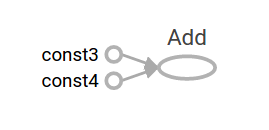
node3 = tf.add(node1, node2)
print("node3:", node3)
print("sess.run(node3):", sess.run(node3))
======================================
node3: Tensor("Add:0", shape=(), dtype=float32)
sess.run(node3): 7.0

TensorBoard screenshot

就像这样，这个图并不是特别引人注目，因为它总是产生一个恒定的结果。可以将图形参数化为接受外部输入，称为placeholder。 占位符是稍后提供值的承诺。

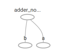
a = tf.placeholder(tf.float32)
b = tf.placeholder(tf.float32)
adder_node = a + b  # + 提供tf.add(a, b)的一个快捷方式

前面的三行有点像函数或lambda，我们在其中定义两个输入参数（a和b），然后对它们进行操作。我们可以通过使用run 方法的feed_dict参数为占位符提供具体值，从而对多个输入进行求值。

print(sess.run(adder_node, {a: 3, b: 4.5}))
print(sess.run(adder_node, {a: [1, 3], b: [2, 4]}))
7.5
[ 3.  7.]

TensorBoard screenshot

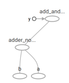
add_and_triple = adder_node * 3.
print(sess.run(add_and_triple, {a: 3, b: 4.5}))
====
22.5

TensorBoard screenshot

在机器学习中，我们通常需要一个可以进行任意输入的模型，比如上面的模型。为了使模型可训练，我们需要修改图形以获得具有相同输入的新输出。 Variables允许我们向图中添加可训练的参数。它们由一个类型和初始值构建而成：

W = tf.Variable([.3], dtype=tf.float32)
b = tf.Variable([-.3], dtype=tf.float32)
x = tf.placeholder(tf.float32)
linear_model = W * x + b

当你调用tf.constant时，常量被初始化，并且它们的值永远不会改变。相比之下，当您调用tf.Variable时，变量不会被初始化。要初始化TensorFlow程序中的所有变量，您必须显式调用特殊操作，如下所示：

init = tf.global_variables_initializer()
sess.run(init)

重要的是要注意到init是TensorFlow子图的句柄，它初始化所有全局变量。在我们调用sess.run之前，变量未初始化。

由于x是一个placeholder，我们可以对x的几个值同时计算linear_model，如下所示：

print(sess.run(linear_model, {x: [1, 2, 3, 4]}))

产生输出

[ 0.          0.30000001  0.60000002  0.90000004]

我们已经创建了一个模型，但我们不知道它有多好。为了评估训练数据模型，我们需要一个y占位符来提供所需的值，我们需要编写一个损失函数。

损失函数用于衡量当前模型距离提供的数据有多远。我们将使用线性回归的标准损失模型，它将当前模型与提供的数据之间的增量的平方相加。 linear_model - y 创建一个向量，其中每个元素都是对应的样本的错误差值。我们调用tf.square来平方该误差。然后，我们使用tf.reduce_sum求和所有平方误差来创建一个单一的标量，它抽取出所有样本的误差：

y = tf.placeholder(tf.float32)
squared_deltas = tf.square(linear_model - y)
loss = tf.reduce_sum(squared_deltas)
print(sess.run(loss, {x: [1, 2, 3, 4], y: [0, -1, -2, -3]}))

产生损失值

23.66

2.2 tf.square()

tf.square( x,
    name=None)
# 计算 x 元素的平方。

2.3 tf.reduce_sum()

压缩求和，一般用于降维

x = tf.constant([[1, 1, 1], [1, 1, 1]])
tf.reduce_sum(x)  # 6求和
tf.reduce_sum(x, 0)  # [2, 2, 2] 按列求和
tf.reduce_sum(x, 1)  # [3, 3] 按照行求和
tf.reduce_sum(x, 1, keepdims=True)  # [[3], [3]] 按照行的维度求和
tf.reduce_sum(x, [0, 1])  # 6 行列求和

2.4 tf.train API

机器学习的完整讨论超出了本教程的范围。但是，TensorFlow提供了优化器，可以缓慢更改每个变量以最大限度地减少损失函数。最简单的优化器是渐变下降。它根据相对于该变量的损失导数的大小来修改每个变量。一般来说，手动计算符号派生是繁琐且容易出错的。因此，TensorFlow可以使用函数tf.gradients自动生成衍生物，只给出模型的描述。为了简单起见，优化程序通常会为您执行此操作。例如，

optimizer = tf.train.GradientDescentOptimizer(0.01)
train = optimizer.minimize(loss)
sess.run(init) # 重置为不正确的默认值。
for i in range(1000):
  sess.run(train, {x: [1, 2, 3, 4], y: [0, -1, -2, -3]})

print(sess.run([W, b]))

得到最终的模型参数：

[array([-0.9999969], dtype=float32), array([ 0.99999082],
 dtype=float32)]

现在我们完成了实际的机器学习！尽管做这种简单的线性回归并不需要太多的TensorFlow核心代码，但更复杂的模型和方法将数据提供给模型需要更多的代码。因此TensorFlow为常见的模式，结构和功能提供更高层次的抽象。我们将在下一节中学习如何使用这些抽象。

2.5 完整的程序

完整的可训练线性回归模型如下所示：

import tensorflow as tf

# Model parameters
W = tf.Variable([.3], dtype=tf.float32)
b = tf.Variable([-.3], dtype=tf.float32)
# Model input and output
x = tf.placeholder(tf.float32)
linear_model = W * x + b
y = tf.placeholder(tf.float32)

# loss
loss = tf.reduce_sum(tf.square(linear_model - y)) # sum of the squares
# optimizer
optimizer = tf.train.GradientDescentOptimizer(0.01)
train = optimizer.minimize(loss)

# training data
x_train = [1, 2, 3, 4]
y_train = [0, -1, -2, -3]
# training loop
init = tf.global_variables_initializer()
sess = tf.Session()
sess.run(init) # reset values to wrong
for i in range(1000):
  sess.run(train, {x: x_train, y: y_train})

# evaluate training accuracy
curr_W, curr_b, curr_loss = sess.run([W, b, loss], {x: x_train, y: y_train})
print("W: %s b: %s loss: %s"%(curr_W, curr_b, curr_loss))

运行时，它会产生

W: [-0.9999969] b: [ 0.99999082] loss: 5.69997e-11

请注意，损失是非常小的数字（非常接近零）。如果你运行这个程序，你的损失可能不完全相同，因为模型是用伪随机值初始化的。

这个更复杂的程序仍然可以在TensorBoard中可视化 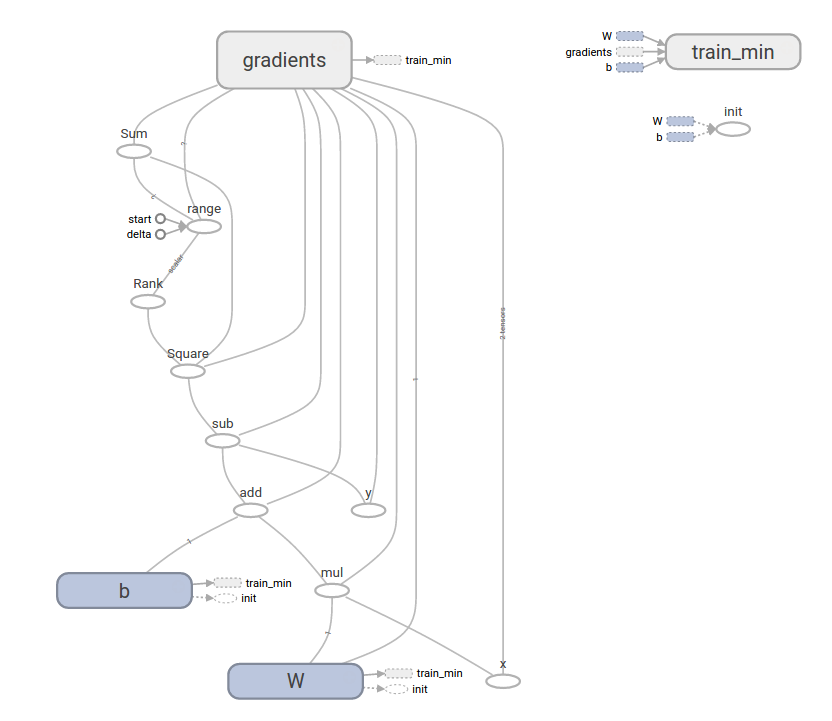TensorBoard final model visualization

2.6 tf.estimator()

tf.estimator is a high-level TensorFlow library that simplifies the mechanics of machine learning, including the following:

运行训练循环
运行评估循环
管理数据集

tf.estimator定义了许多通用模型。

可以用于简化线性回归程序

import tensorflow as tf
# NumPy 经常用于加载、操作和预处理数据。
import numpy as np

# 声明特征列表。 我们只有一个数字特征。 有许多
# 其它类型的列，它们更复杂而且更有用。
feature_columns = [tf.feature_column.numeric_column("x", shape=[1])]

# An estimator is the front end to invoke training (fitting) and evaluation
# (inference). 有许多预定义类型，如线性回归、
# 线性分类以及许多神经网络分类器和回归器。
# 下面的代码给出一个estimator，它实现线性回归。
estimator = tf.estimator.LinearRegressor(feature_columns=feature_columns)

# TensorFlow 提供许多辅助方法来读取和建立数据集。
# 这里我们使用两个数据集：一个用于训练，一个用于评估。
# 我们必须告诉函数
# 我们想要数据的多少个batch(num_epochs)以及每个batch的大小。
x_train = np.array([1., 2., 3., 4.])
y_train = np.array([0., -1., -2., -3.])
x_eval = np.array([2., 5., 8., 1.])
y_eval = np.array([-1.01, -4.1, -7, 0.])
input_fn = tf.estimator.inputs.numpy_input_fn(
    {"x": x_train}, y_train, batch_size=4, num_epochs=None, shuffle=True)
train_input_fn = tf.estimator.inputs.numpy_input_fn(
    {"x": x_train}, y_train, batch_size=4, num_epochs=1000, shuffle=False)
eval_input_fn = tf.estimator.inputs.numpy_input_fn(
    {"x": x_eval}, y_eval, batch_size=4, num_epochs=1000, shuffle=False)

# We can invoke 1000 training steps by invoking the  method and passing the
# training data set.
estimator.train(input_fn=input_fn, steps=1000)

# 这里我们评估我们的模型表现如何
train_metrics = estimator.evaluate(input_fn=train_input_fn)
eval_metrics = estimator.evaluate(input_fn=eval_input_fn)
print("train metrics: %r"% train_metrics)
print("eval metrics: %r"% eval_metrics)
运行时，它会产生

train metrics: {'loss': 1.2712867e-09, 'global_step': 1000}
eval metrics: {'loss': 0.0025279333, 'global_step': 1000}
请注意我们的评估数据的损失有点高，但仍然接近于零。 这意味着我们正在正确地学习。

定制模型
tf.estimator不会将您锁定到其预定义的模型中。 假设我们想创建一个没有内置到TensorFlow中的自定义模型。 我们仍然可以维持对数据集、feeding、训练等的高层抽象。 tf.estimator。 为了说明，我们将使用我们对较低级别TensorFlow API的了解，展示如何实现我们自己的与LinearRegressor等效模型。

To define a custom model that works with tf.estimator, we need to use tf.estimator.Estimator. tf.estimator.LinearRegressor is actually a sub-class of tf.estimator.Estimator. 不用子类化Estimator，我们仅仅提供Estimator一个函数model_fn，该函数告诉tf.estimator如何评估预测、训练步骤和损失。 代码如下：

import numpy as np
import tensorflow as tf

# 声明特征列表，我们只有一个实数特征
def model_fn(features, labels, mode):
  # 构建一个线性模型并预测值
  W = tf.get_variable("W", [1], dtype=tf.float64)
  b = tf.get_variable("b", [1], dtype=tf.float64)
  y = W * features['x'] + b
  # Loss sub-graph
  loss = tf.reduce_sum(tf.square(y - labels))
  # Training sub-graph
  global_step = tf.train.get_global_step()
  optimizer = tf.train.GradientDescentOptimizer(0.01)
  train = tf.group(optimizer.minimize(loss),
                   tf.assign_add(global_step, 1))
  # EstimatorSpec connects subgraphs we built to the
  # appropriate functionality.
  return tf.estimator.EstimatorSpec(
      mode=mode,
      predictions=y,
      loss=loss,
      train_op=train)

estimator = tf.estimator.Estimator(model_fn=model_fn)
# define our data sets
x_train = np.array([1., 2., 3., 4.])
y_train = np.array([0., -1., -2., -3.])
x_eval = np.array([2., 5., 8., 1.])
y_eval = np.array([-1.01, -4.1, -7, 0.])
input_fn = tf.estimator.inputs.numpy_input_fn(
    {"x": x_train}, y_train, batch_size=4, num_epochs=None, shuffle=True)
train_input_fn = tf.estimator.inputs.numpy_input_fn(
    {"x": x_train}, y_train, batch_size=4, num_epochs=1000, shuffle=False)
eval_input_fn = tf.estimator.inputs.numpy_input_fn(
    {"x": x_eval}, y_eval, batch_size=4, num_epochs=1000, shuffle=False)

# train
estimator.train(input_fn=input_fn, steps=1000)
# Here we evaluate how well our model did.
train_metrics = estimator.evaluate(input_fn=train_input_fn)
eval_metrics = estimator.evaluate(input_fn=eval_input_fn)
print("train metrics: %r"% train_metrics)
print("eval metrics: %r"% eval_metrics)

import tensorflow as tf
# NumPy 经常用于加载、操作和预处理数据。
import numpy as np

# 声明特征列表。 我们只有一个数字特征。 有许多
# 其它类型的列，它们更复杂而且更有用。
feature_columns = [tf.feature_column.numeric_column("x", shape=[1])]

# An estimator is the front end to invoke training (fitting) and evaluation
# (inference). 有许多预定义类型，如线性回归、
# 线性分类以及许多神经网络分类器和回归器。
# 下面的代码给出一个estimator，它实现线性回归。
estimator = tf.estimator.LinearRegressor(feature_columns=feature_columns)

# TensorFlow 提供许多辅助方法来读取和建立数据集。
# 这里我们使用两个数据集：一个用于训练，一个用于评估。
# 我们必须告诉函数
# 我们想要数据的多少个batch(num_epochs)以及每个batch的大小。
x_train = np.array([1., 2., 3., 4.])
y_train = np.array([0., -1., -2., -3.])
x_eval = np.array([2., 5., 8., 1.])
y_eval = np.array([-1.01, -4.1, -7, 0.])
input_fn = tf.estimator.inputs.numpy_input_fn(
    {"x": x_train}, y_train, batch_size=4, num_epochs=None, shuffle=True)
train_input_fn = tf.estimator.inputs.numpy_input_fn(
    {"x": x_train}, y_train, batch_size=4, num_epochs=1000, shuffle=False)
eval_input_fn = tf.estimator.inputs.numpy_input_fn(
    {"x": x_eval}, y_eval, batch_size=4, num_epochs=1000, shuffle=False)

# We can invoke 1000 training steps by invoking the  method and passing the
# training data set.
estimator.train(input_fn=input_fn, steps=1000)

# 这里我们评估我们的模型表现如何
train_metrics = estimator.evaluate(input_fn=train_input_fn)
eval_metrics = estimator.evaluate(input_fn=eval_input_fn)
print("train metrics: %r"% train_metrics)
print("eval metrics: %r"% eval_metrics)

运行时，它会产生

train metrics: {'loss': 1.2712867e-09, 'global_step': 1000}
eval metrics: {'loss': 0.0025279333, 'global_step': 1000}

请注意我们的评估数据的损失有点高，但仍然接近于零。这意味着我们正在正确地学习。

2.7 定制模型

tf.estimator不会将您锁定到其预定义的模型中。假设我们想创建一个没有内置到TensorFlow中的自定义模型。我们仍然可以维持对数据集、feeding、训练等的高层抽象。 tf.estimator。为了说明，我们将使用我们对较低级别TensorFlow API的了解，展示如何实现我们自己的与LinearRegressor等效模型。

To define a custom model that works with tf.estimator, we need to use tf.estimator.Estimator.tf.estimator.LinearRegressor is actually a sub-class of tf.estimator.Estimator. 不用子类化Estimator，我们仅仅提供Estimator一个函数model_fn，该函数告诉tf.estimator如何评估预测、训练步骤和损失。代码如下：

import numpy as np
import tensorflow as tf

# 声明特征列表，我们只有一个实数特征
def model_fn(features, labels, mode):
  # 构建一个线性模型并预测值
  W = tf.get_variable("W", [1], dtype=tf.float64)
  b = tf.get_variable("b", [1], dtype=tf.float64)
  y = W * features['x'] + b
  # Loss sub-graph
  loss = tf.reduce_sum(tf.square(y - labels))
  # Training sub-graph
  global_step = tf.train.get_global_step()
  optimizer = tf.train.GradientDescentOptimizer(0.01)
  train = tf.group(optimizer.minimize(loss),
                   tf.assign_add(global_step, 1))
  # EstimatorSpec connects subgraphs we built to the
  # appropriate functionality.
  return tf.estimator.EstimatorSpec(
      mode=mode,
      predictions=y,
      loss=loss,
      train_op=train)

estimator = tf.estimator.Estimator(model_fn=model_fn)
# define our data sets
x_train = np.array([1., 2., 3., 4.])
y_train = np.array([0., -1., -2., -3.])
x_eval = np.array([2., 5., 8., 1.])
y_eval = np.array([-1.01, -4.1, -7, 0.])
input_fn = tf.estimator.inputs.numpy_input_fn(
    {"x": x_train}, y_train, batch_size=4, num_epochs=None, shuffle=True)
train_input_fn = tf.estimator.inputs.numpy_input_fn(
    {"x": x_train}, y_train, batch_size=4, num_epochs=1000, shuffle=False)
eval_input_fn = tf.estimator.inputs.numpy_input_fn(
    {"x": x_eval}, y_eval, batch_size=4, num_epochs=1000, shuffle=False)

# train
estimator.train(input_fn=input_fn, steps=1000)
# Here we evaluate how well our model did.
train_metrics = estimator.evaluate(input_fn=train_input_fn)
eval_metrics = estimator.evaluate(input_fn=eval_input_fn)
print("train metrics: %r"% train_metrics)
print("eval metrics: %r"% eval_metrics)

运行时，它会产生

train metrics: {'loss': 1.227995e-11, 'global_step': 1000}
eval metrics: {'loss': 0.01010036, 'global_step': 1000}

请注意，自定义model_fn()函数的内容与我们采用底层API的手动模型训练循环非常相似。

2.8 tf.train.Saver()

管理模型中的所有变量。可以将变量保存到检查点文件中。

# Create some variables.
v1 = tf.get_variable("v1", shape=[3], initializer = tf.zeros_initializer)
v2 = tf.get_variable("v2", shape=[5], initializer = tf.zeros_initializer)

inc_v1 = v1.assign(v1+1)
dec_v2 = v2.assign(v2-1)

# Add an op to initialize the variables.
init_op = tf.global_variables_initializer()

# Add ops to save and restore all the variables.
saver = tf.train.Saver()

# Later, launch the model, initialize the variables, do some work, and save the
# variables to disk.
with tf.Session() as sess:
  sess.run(init_op)
  # Do some work with the model.
  inc_v1.op.run()
  dec_v2.op.run()
  # Save the variables to disk.
  save_path = saver.save(sess, "/tmp/model.ckpt")
  print("Model saved in path: %s" % save_path)

2.9 tf.logging.set_verbosity日志消息

在tensorflow中有函数可以直接log打印，这个跟ROS系统中打印函数差不多。

TensorFlow使用五个不同级别的日志消息。按照上升的顺序，它们是DEBUG，INFO，WARN，ERROR和FATAL。当您在任何这些级别配置日志记录时，TensorFlow将输出与该级别相对应的所有日志消息以及所有级别的严重级别。例如，如果设置了ERROR的日志记录级别，则会收到包含ERROR和FATAL消息的日志输出，如果设置了一个DEBUG级别，则会从所有五个级别获取日志消息。 # 默认情况下，TENSFlow在WARN的日志记录级别进行配置，但是在跟踪模型训练时，您需要将级别调整为INFO，这将提供适合操作正在进行的其他反馈。

2.10 tf.app.run()

理flag解析，然后执行main函数，那么flag解析是什么意思呢？诸如这样的：

tf.app.flags.DEFINE_boolean("self_test", False, "True if running a self test.")
tf.app.flags.DEFINE_boolean('use_fp16', False,
                            "Use half floats instead of full floats if True.")
FLAGS = tf.app.flags.FLAGS

如果你的代码中的入口函数不叫main()，而是一个其他名字的函数，如test()，则你应该这样写入口tf.app.run(test())
如果你的代码中的入口函数叫main()，则你就可以把入口写成tf.app.run()

2.11 tf.device(dev)

使用 tf.device() 指定模型运行的具体设备，可以指定运行在GPU还是CUP上，以及哪块GPU上。

设置使用GPU

使用 tf.device(‘/gpu:1’) 指定Session在第二块GPU上运行

2.12 InteractiveSession

Tensorflow依赖于一个高效的C++后端来进行计算，与后端的连接叫做session。使用TensorFlow程序的流程是先创建一个图，然后在session中启动它。

import tensorflow as tf
sess = tf.InteractiveSession()

2.13 tf.metrics.accuracy

tf.metrics.accuracy(
    labels,
    predictions,
    weights=None,
    metrics_collections=None,
    updates_collections=None,
    name=None
)

Calculates how often predictions matches labels.

The accuracy function creates two local variables, total and count that are used to compute the frequency with which predictions matches labels. This frequency is ultimately returned as accuracy: an idempotent operation that simply divides total by count

2.14 tf.random_normal()

tf.random_normal()函数用于从服从指定正太分布的数值中取出指定个数的值。

tf.random_normal(shape, mean=0.0, stddev=1.0, dtype=tf.float32, seed=None, name=None)

shape: 输出张量的形状，必选
mean: 正态分布的均值，默认为0
stddev: 正态分布的标准差，默认为1.0
dtype: 输出的类型，默认为tf.float32
seed: 随机数种子，是一个整数，当设置之后，每次生成的随机数都一样
name: 操作的名称 ~~~python # -*- coding: utf-8 -*-) import tensorflow as tf

w1 = tf.Variable(tf.random_normal([2, 3], stddev=1, seed=1))

with tf.Session() as sess: sess.run(tf.global_variables_initializer()) # sess.run(tf.initialize_all_variables()) #比较旧一点的初始化变量方法 print w1 print sess.run(w1)

**输出**

~~~python
<tf.Variable 'Variable:0' shape=(2, 3) dtype=float32_ref>
[[-0.81131822  1.48459876  0.06532937]
 [-2.4427042   0.0992484   0.59122431]]

X = tf.random_normal(shape=[3, 5, 6], dtype=tf.float32)

输出

[[[ 1.2145256  -1.1560208  -1.093731    1.2256579   0.7898847
    0.4307395 ]
  [ 0.40822104  1.129571    1.5324206   1.0552545  -2.2940836
    0.6523705 ]
  [-1.7757286   1.6769009  -2.4429555  -1.0986998   1.4876577
   -0.5120297 ]
  [ 0.84597296  0.08493174 -0.13421828  0.8137087   0.10831776
    0.6971543 ]
  [-1.5157102   0.5615479   1.5183837   1.2744774  -0.50404435
   -0.01050083]]

 [[-0.16702758 -0.21784598  1.3655689  -0.5927149   0.00593981
   -0.44541496]
  [ 0.9233799   0.8480989   2.1650398  -1.1013446   2.6040213
   -0.3909698 ]
  [ 0.43016607 -2.2001355   0.88257426  0.8560082   1.4979376
    0.18180591]
  [-0.45241094  0.32941505 -0.90290606 -1.5022529   0.3843127
   -0.48287177]
  [-1.0534667  -0.23643473 -0.20744231  0.83963126  0.1148954
   -0.1779806 ]]

 [[ 0.14691043 -1.522594    0.43237835  1.7798514   0.866155
   -1.5195131 ]
  [ 0.8440296  -1.4065892   0.88740623  0.18301357  1.3123437
   -1.456079  ]
  [ 0.10538957 -0.2888947  -0.6975345  -0.48583674 -0.6506234
   -0.30639789]
  [ 1.8601152   1.2282892  -0.5889973  -0.95935255 -0.33233717
    0.28872928]
  [-1.1773086   0.05818317 -1.3115891  -0.22604029  0.17960498
   -1.4679621 ]]]

2.15 cell.zero_state

init_state = cell.zero_state(3, dtype=tf.float32)

结果

[[0. 0. 0. 0. 0. 0. 0. 0. 0. 0.]
 [0. 0. 0. 0. 0. 0. 0. 0. 0. 0.]
 [0. 0. 0. 0. 0. 0. 0. 0. 0. 0.]]

2.16 tf.nn.rnn_cell.GRUCell

tf.nn.rnn_cell.GRUCell(num_units, input_size=None, activation=<function tanh>).num_units
就是隐层神经元的个数，默认的activation就是tanh，你也可以自己定义，但是一般都不会去修改。
这个函数的主要的参数就是num_units。

2.17 tf.nn.dynamic_rnn

tf.nn.dynamic_rnn(
    cell,
    inputs,
    sequence_length=None,
    initial_state=None,
    dtype=None,
    parallel_iterations=None,
    swap_memory=False,
    time_major=False,
    scope=None
)

batch_size是输入的这批数据的数量，max_time就是这批数据中序列的最长长度，如果输入的三个句子，那max_time对应的就是最长句子的单词数量，cell.output_size其实就是rnn cell中神经元的个数。

output

是一个tensor
如果time_major==True，outputs形状为 [max_time, batch_size, cell.output_size ]（要求rnn输入与rnn输出形状保持一致）
如果time_major==False（默认），outputs形状为 [ batch_size, max_time, cell.output_size ]

state

是一个tensor
state是最终的状态，也就是序列中最后一个cell输出的状态
一般情况下state的形状为 [batch_size, cell.output_size ]，但当输入的cell为BasicLSTMCell时，state的形状为[2，batch_size, cell.output_size ]，其中2也对应着LSTM中的cell state和hidden state

2.18 tf.reshape

images = np.array([1, 2, 3, 4, 5, 6, 7, 8, 9, 0])  
d = images.reshape((-1, 1, 2, 1))                  
print(d)                                       

输出结果：

[[[[1]
   [2]]]
 [[[3]
   [4]]]
 [[[5]
   [6]]]
 [[[7]
   [8]]]
 [[[9]
   [0]]]]

解释：这个函数的作用是对tensor的维度进行重新组合。给定一个tensor，这个函数会返回数据维度是shape的一个新的tensor，但是tensor里面的元素不变。如果shape是一个特殊值[-1]，那么tensor将会变成一个扁平的一维tensor。如果shape是一个一维或者更高的tensor，那么输入的tensor将按照这个shape进行重新组合，但是重新组合的tensor和原来的tensor的元素是必须相同的。

使用例子：

#!/usr/bin/env python
# -*- coding: utf-8 -*-

import tensorflow as tf 
import numpy as np 

sess = tf.Session()
data = tf.constant([[[1, 1, 1], [2, 2, 2]], [[3, 3, 3], [4, 4, 4]]])
print sess.run(data)
print sess.run(tf.shape(data))
d = tf.reshape(data, [-1])
print sess.run(d)
d = tf.reshape(data, [3, 4])
print sess.run(d)

输入参数：

tensor: 一个Tensor。
shape: 一个Tensor，数据类型是int32，定义输出数据的维度。
name:（可选）为这个操作取一个名字。

输出参数：

一个Tensor，数据类型和输入数据相同。

2.19 tf.clip_by_global_norm

tf.clip_by_global_norm(t_list, clip_norm, use_norm=None, name=None)

通过权重梯度的总和的比率来截取多个张量的值。 t_list 是梯度张量， clip_norm 是截取的比率, 这个函数返回截取过的梯度张量和一个所有张量的全局范数。

t_list[i] 的更新公式如下:

t_list[i] * clip_norm / max(global_norm, clip_norm)

其中global_norm = sqrt(sum([l2norm(t)**2 for t in t_list])) global_norm 是所有梯度的平方和，如果 clip_norm > global_norm ，就不进行截取。但是这个函数的速度比clip_by_norm() 要慢，因为在截取之前所有的参数都要准备好。其他实现的函数还有这些

2.20 tf.pad

作用：填充

pad(
    tensor,
    paddings,
    mode='CONSTANT',
    name=None
)

tensor是要填充的张量 padings 也是一个张量，代表每一维填充多少行/列，但是有一个要求它的rank一定要和tensor的rank是一样的

mode 可以取三个值，分别是”CONSTANT” ,”REFLECT”,”SYMMETRIC”

mode=”CONSTANT” 是填充0

mode=”REFLECT”是映射填充，上下（1维）填充顺序和paddings是相反的，左右（零维）顺序补齐

mode=”SYMMETRIC”是对称填充，上下（1维）填充顺序是和paddings相同的，左右（零维）对称补齐

2.21 tf.concat

tf.concat(
    values,
    axis,
    name='concat'
)

values应该是一个tensor的list或者tuple。
axis则是我们想要连接的维度。
tf.concat返回的是连接后的tensor。

2.22 tf.cast

tf.cast(
    x,
    dtype,
    name=None
)

tf.cast可以改变tensor的数据类型

2.23 tf.add

x = tf.constant(8, name="x_const")
y = tf.constant(5, name="y_const")
sum = tf.add(x, y, name="x_y_sum")

三、模型的训练

3.1 定义指标

定义指标，衡量模型是好的还是坏的
指标称为成本（成本）或者损失（loss）
然后需要最小化这个指标

3.2 交叉熵

一个非常漂亮的成本函数
产生于信息论里面的信息压缩编码技术，后来演变称为机器学习中的重要技术手段

y：预测的概率分布

y’：实际的分布（eg：one-hot）
为了计算交叉熵，需要添加一个新的占位符
```
y_ = tf.placeholder("float", [None,10])
```
计算交叉熵
```
cross_entropy = -tf.reduce_sum(y_*tf.log(y))
```
首先，用 tf.log 计算 y 的每个元素的对数。接下来，我们把 y_ 的每一个元素和 tf.log(y_) 的对应元素相乘。最后，用 tf.reduce_sum 计算张量的所有元素的总和。（注意，这里的交叉熵不仅仅用来衡量单一的一对预测和真实值，而是所有100幅图片的交叉熵的总和。对于100个数据点的预测表现比单一数据点的表现能更好地描述我们的模型的性能。

3.3 自动使用反向传播

确定你的变量是如何影响你想要最小化的那个成本值
TensorFlow会用你选择的优化算法来不断地修改变量以降低成本。
```
train_step = tf.train.GradientDescentOptimizer(0.01).minimize(cross_entropy)
```
在这里，我们要求TensorFlow用梯度下降算法（gradient descent algorithm）以0.01的学习速率最小化交叉熵。梯度下降算法（gradient descent algorithm）是一个简单的学习过程，TensorFlow只需将每个变量一点点地往使成本不断降低的方向移动。当然TensorFlow也提供了其他许多优化算法：只要简单地调整一行代码就可以使用其他的算法。

3.4 初始化变量

现在，我们已经设置好了我们的模型。在运行计算之前，我们需要添加一个操作来初始化我们创建的变量：

init = tf.initialize_all_variables()

在一个Session里面启动我们的模型，并且初始化变量：

sess = tf.Session()
sess.run(init)

3.5 设置训练次数

eg：然后开始训练模型，这里我们让模型循环训练1000次！

for i in range(1000):
  batch_xs, batch_ys = mnist.train.next_batch(100)
  sess.run(train_step, feed_dict={x: batch_xs, y_: batch_ys})

该循环的每个步骤，会随机抓取训练数据中的100个批处理数据点。
然后用这个数据点，作为参数替换之前的占位符来运行train_step
使用一小部分的随机数据来进行训练被称为随机训练（stochastic training）- 在这里更确切的说是随机梯度下降训练。
在理想情况下，我们希望用我们所有的数据来进行每一步的训练，因为这能给我们更好的训练结果，但显然这需要很大的计算开销。
所以，每一次训练我们可以使用不同的数据子集，这样做既可以减少计算开销，又可以最大化地学习到数据集的总体特性。

四、模型评估

4.1 找出预测正确的标签

tf.argmax 是一个非常有用的函数，它能给出某个tensor对象在某一维上的其数据最大值所在的索引值。
由于标签向量是由0,1组成，因此最大值1所在的索引位置就是类别标签，比如tf.argmax(y,1)返回的是模型对于任一输入x预测到的标签值，而 tf.argmax(y_,1) 代表正确的标签，我们可以用 tf.equal来检测我们的预测是否真实标签匹配(索引位置一样表示匹配)。
```
correct_prediction = tf.equal(tf.argmax(y,1), tf.argmax(y_,1))
```
上述代码，输出一组布尔值，为了确定正确预测项的比例，可以把布尔值转换成浮点数，然后再去平均值。
比如，[True, False, True, True] 会变成 [1,0,1,1] ，取平均值后得到 0.75.
```
accuracy = tf.reduce_mean(tf.cast(correct_prediction, "float"))
```

将学习到的模型在测试数据集上看下正确率

print sess.run(accuracy, feed_dict={x: mnist.test.images, y_: mnist.test.labels})

print accuracy.eval(feed_dict={x: mnist.test.images, y_: mnist.test.labels})

五、多层卷积神经网络

5.1 权重初始化

首先需要创建大量的权重和偏置项
权重在初始化时应该加入少量的噪声来打破对称性以及避免0梯度
由于我们使用的是ReLU神经元，因此比较好的做法是用一个较小的正数来初始化偏置项，以避免神经元节点输出恒为0的问题（dead neurons）

为了不在建立模型的时候反复做初始化操作，我们定义两个函数用于初始化。

def weight_variable(shape):
  initial = tf.truncated_normal(shape, stddev=0.1)
  return tf.Variable(initial)
  
def bias_variable(shape):
  initial = tf.constant(0.1, shape=shape)
  return tf.Variable(initial)

5.2 卷积和池化

卷积使用1步长（stride size），0边距（padding size）的模板，保证输出和输入是同一个大小。我们的池化用简单传统的2x2大小的模板做max pooling。为了代码更简洁，我们把这部分抽象成一个函数。

def conv2d(x, W):
  return tf.nn.conv2d(x, W, strides=[1, 1, 1, 1], padding='SAME')
  
def max_pool_2x2(x):
  return tf.nn.max_pool(x, ksize=[1, 2, 2, 1],
                        strides=[1, 2, 2, 1], padding='SAME')

5.3 第一层卷积

一个卷积接一个max pooling 完成
卷积在每个5x5的patch中算出32个特征。卷积的权重张量形状是[5, 5, 1, 32]，前两个维度是patch的大小，接着是输入的通道数目，最后是输出的通道数目。
每一个输出通道都有一个对应的偏置量
```
W_conv1 = weight_variable([5, 5, 1, 32])
b_conv1 = bias_variable([32])
```
为了用这一层，我们把x变成一个4d向量，其第2、第3维对应图片的宽、高，最后一维代表图片的颜色通道数(因为是灰度图所以这里的通道数为1，如果是rgb彩色图，则为3)。
```
x_image = tf.reshape(x, [-1,28,28,1])
```
We then convolve x_image with the weight tensor, add the bias, apply the ReLU function, and finally max pool. 我们把x_image和权值向量进行卷积，加上偏置项，然后应用ReLU激活函数，最后进行max pooling。
```
h_conv1 = tf.nn.relu(conv2d(x_image, W_conv1) + b_conv1)
h_pool1 = max_pool_2x2(h_conv1)
```

5.4 第二层卷积

第二层中，每个5x5的patch会得到64个特征

W_conv2 = weight_variable([5, 5, 32, 64])
b_conv2 = bias_variable([64])
h_conv2 = tf.nn.relu(conv2d(h_pool1, W_conv2) + b_conv2)
h_pool2 = max_pool_2x2(h_conv2)

5.5 密集连接层

现在，图片尺寸减小到7x7，我们加入一个有1024个神经元的全连接层，用于处理整个图片。我们把池化层输出的张量reshape成一些向量，乘上权重矩阵，加上偏置，然后对其使用ReLU。
```
W_fc1 = weight_variable([7 * 7 * 64, 1024])
b_fc1 = bias_variable([1024])
  
h_pool2_flat = tf.reshape(h_pool2, [-1, 7*7*64])
h_fc1 = tf.nn.relu(tf.matmul(h_pool2_flat, W_fc1) + b_fc1)
```

5.6 Dropout

为了减少过拟合，我们在输出层之前加入dropout
用一个placeholder来代表一个神经元的输出在dropout中保持不变的概率。这样我们可以在训练过程中启用dropout，在测试过程中关闭dropout。
TensorFlow的tf.nn.dropout操作除了可以屏蔽神经元的输出外，还会自动处理神经元输出值的scale。所以用dropout的时候可以不用考虑scale。
```
keep_prob = tf.placeholder("float")
h_fc1_drop = tf.nn.dropout(h_fc1, keep_prob)
```

5.7 输出层

添加一个softmax层，就像前面的单层softmax regression一样

W_fc2 = weight_variable([1024, 10])
b_fc2 = bias_variable([10])
  
y_conv=tf.nn.softmax(tf.matmul(h_fc1_drop, W_fc2) + b_fc2)

5.8 训练和评估模型

cross_entropy = -tf.reduce_sum(y_*tf.log(y_conv))
train_step = tf.train.AdamOptimizer(1e-4).minimize(cross_entropy)
correct_prediction = tf.equal(tf.argmax(y_conv,1), tf.argmax(y_,1))
accuracy = tf.reduce_mean(tf.cast(correct_prediction, "float"))
sess.run(tf.initialize_all_variables())
for i in range(20000):
  batch = mnist.train.next_batch(50)
  if i%100 == 0:
    train_accuracy = accuracy.eval(feed_dict={
        x:batch[0], y_: batch[1], keep_prob: 1.0})
    print "step %d, training accuracy %g"%(i, train_accuracy)
  train_step.run(feed_dict={x: batch[0], y_: batch[1], keep_prob: 0.5})

print "test accuracy %g"%accuracy.eval(feed_dict={
    x: mnist.test.images, y_: mnist.test.labels, keep_prob: 1.0})

##六、简单案例

6.1 两个常数相加

import tensorflow as tf
g = tf.Graph()
with g.as_default():
  x = tf.constant(8, name="x_const")
  y = tf.constant(5, name="y_const")
  sum = tf.add(x, y, name="x_y_sum")
  
  # Task 1: Define a third scalar integer constant z.
  z = tf.constant(4, name="z_const")
  # Task 2: Add z to `sum` to yield a new sum.
  new_sum = tf.add(sum, z, name="x_y_z_sum")

  # Now create a session.
  # The session will run the default graph.
  with tf.Session() as sess:
    # Task 3: Ensure the program yields the correct grand total.
    print(new_sum.eval())

6.2 定义变量

# 变量定义
def var_test():
  state = tf.Variable(0, name="counter")
  input1 = tf.constant(3.0)
  input1 = tf.placeholder(tf.float32)
  input2 = tf.placeholder(tf.float32)
  output = tf.matmul(input1, input2)
  with tf.Session() as sess:
    print(sess.run([output], feed_dict={input1: [7.], input2: [2.]}))

if __name__ == '__main__':
    # graph()
  var_test()

出现问题

WARNING:tensorflow:From /Users/stone/anaconda3/envs/tensorflow_36/lib/python3.6/site-packages/tensorflow/python/framework/op_def_library.py:263: colocate_with (from tensorflow.python.framework.ops) is deprecated and will be removed in a future version.
Instructions for updating:
Colocations handled automatically by placer.
2019-11-03 10:13:33.757337: I tensorflow/core/platform/cpu_feature_guard.cc:141] Your CPU supports instructions that this TensorFlow binary was not compiled to use: SSE4.1 SSE4.2 AVX AVX2 FMA
2019-11-03 10:13:33.757636: I tensorflow/core/common_runtime/process_util.cc:71] Creating new thread pool with default inter op setting: 8. Tune using inter_op_parallelism_threads for best performance.
Traceback (most recent call last):
  File "/Users/stone/anaconda3/envs/tensorflow_36/lib/python3.6/site-packages/tensorflow/python/client/session.py", line 1334, in _do_call
    return fn(*args)
  File "/Users/stone/anaconda3/envs/tensorflow_36/lib/python3.6/site-packages/tensorflow/python/client/session.py", line 1319, in _run_fn
    options, feed_dict, fetch_list, target_list, run_metadata)
  File "/Users/stone/anaconda3/envs/tensorflow_36/lib/python3.6/site-packages/tensorflow/python/client/session.py", line 1407, in _call_tf_sessionrun
    run_metadata)
tensorflow.python.framework.errors_impl.InvalidArgumentError: lhs and rhs ndims must be >= 2: 1
	 [[]]

During handling of the above exception, another exception occurred:

Traceback (most recent call last):
  File "/Users/stone/PycharmProjects/ocr_Correction/test/test.py", line 28, in <module>
    var_test()
  File "/Users/stone/PycharmProjects/ocr_Correction/test/test.py", line 24, in var_test
    print(sess.run([output], feed_dict={input1: [7.], input2: [2.]}))
  File "/Users/stone/anaconda3/envs/tensorflow_36/lib/python3.6/site-packages/tensorflow/python/client/session.py", line 929, in run
    run_metadata_ptr)
  File "/Users/stone/anaconda3/envs/tensorflow_36/lib/python3.6/site-packages/tensorflow/python/client/session.py", line 1152, in _run
    feed_dict_tensor, options, run_metadata)
  File "/Users/stone/anaconda3/envs/tensorflow_36/lib/python3.6/site-packages/tensorflow/python/client/session.py", line 1328, in _do_run
    run_metadata)
  File "/Users/stone/anaconda3/envs/tensorflow_36/lib/python3.6/site-packages/tensorflow/python/client/session.py", line 1348, in _do_call
    raise type(e)(node_def, op, message)
tensorflow.python.framework.errors_impl.InvalidArgumentError: lhs and rhs ndims must be >= 2: 1
	 [[node MatMul (defined at /Users/stone/PycharmProjects/ocr_Correction/test/test.py:22) ]]

Caused by op 'MatMul', defined at:
  File "/Users/stone/PycharmProjects/ocr_Correction/test/test.py", line 28, in <module>
    var_test()
  File "/Users/stone/PycharmProjects/ocr_Correction/test/test.py", line 22, in var_test
    output = tf.matmul(input1, input2)
  File "/Users/stone/anaconda3/envs/tensorflow_36/lib/python3.6/site-packages/tensorflow/python/ops/math_ops.py", line 2417, in matmul
    a, b, adj_x=adjoint_a, adj_y=adjoint_b, name=name)
  File "/Users/stone/anaconda3/envs/tensorflow_36/lib/python3.6/site-packages/tensorflow/python/ops/gen_math_ops.py", line 1423, in batch_mat_mul
    "BatchMatMul", x=x, y=y, adj_x=adj_x, adj_y=adj_y, name=name)
  File "/Users/stone/anaconda3/envs/tensorflow_36/lib/python3.6/site-packages/tensorflow/python/framework/op_def_library.py", line 788, in _apply_op_helper
    op_def=op_def)
  File "/Users/stone/anaconda3/envs/tensorflow_36/lib/python3.6/site-packages/tensorflow/python/util/deprecation.py", line 507, in new_func
    return func(*args, **kwargs)
  File "/Users/stone/anaconda3/envs/tensorflow_36/lib/python3.6/site-packages/tensorflow/python/framework/ops.py", line 3300, in create_op
    op_def=op_def)
  File "/Users/stone/anaconda3/envs/tensorflow_36/lib/python3.6/site-packages/tensorflow/python/framework/ops.py", line 1801, in __init__
    self._traceback = tf_stack.extract_stack()

InvalidArgumentError (see above for traceback): lhs and rhs ndims must be >= 2: 1
	 [[node MatMul (defined at /Users/stone/PycharmProjects/ocr_Correction/test/test.py:22) ]]

参考网址

https://www.jianshu.com/p/e5076a56946c
https://yiyibooks.cn/yiyi/tensorflow_13/get_started/get_started.html
https://blog.csdn.net/u010960155/article/details/81707498【tf.nn.dynamic_rnn】

一、 参数介绍

1. 1 epoch，batch size，iteration

1.2 Tensor

1.3 计算图

1.3 占位符

1.4 变量

1.5 类别预测与损失函数

1.6 训练模型

1.7 评估模型

1.8 dropout

二、 相关函数

2.1 tf.placeholder()

2.2 tf.square()

2.3 tf.reduce_sum()

2.4 tf.train API

2.5 完整的程序

2.6 tf.estimator()

2.7 定制模型

2.8 tf.train.Saver()

2.9 tf.logging.set_verbosity日志消息

2.10 tf.app.run()

2.11 tf.device(dev)

2.12 InteractiveSession

2.13 tf.metrics.accuracy

2.14 tf.random_normal()

2.15 cell.zero_state

2.16 tf.nn.rnn_cell.GRUCell

2.17 tf.nn.dynamic_rnn

output

state

2.18 tf.reshape

2.19 tf.clip_by_global_norm

2.20 tf.pad

2.21 tf.concat

2.22 tf.cast

2.23 tf.add

三、模型的训练

3.1 定义指标

3.2 交叉熵

3.3 自动使用反向传播

3.4 初始化变量

3.5 设置训练次数

四、模型评估

4.1 找出预测正确的标签

五、多层卷积神经网络

5.1 权重初始化

5.2 卷积和池化

5.3 第一层卷积

5.4 第二层卷积

5.5 密集连接层

5.6 Dropout

5.7 输出层

5.8 训练和评估模型

6.1 两个常数相加

6.2 定义变量

参考网址

一、参数介绍

二、相关函数