2018-08-01-逻辑回归

2018-08-01 | 阅读：次

b站上一个例子：

数据集

step1:加载文件

import numpy as np
import matplotlib.pyplot as plt


#def loaddata
def loaddata(filename):
    file = open(filename)
    x = []
    y = []
    for line in file.readlines():
        line = line.strip().split()
        x.append([float(line[0]), float(line[1])])
        y.append(float(line[-1]))
    #将列表格式变成为矩阵的格式
    xmat = np.mat(x)
    ymat = np.mat(y)
    file.close()
    return xmat, ymat


#implement
xmat, ymat = loaddata('ytb_lr.txt')
print('xmat:', xmat, xmat.shape)
print('ymat:', ymat, ymat.shape)

运行结果：

D:\1b\Anoconda\setup\set\python.exe E:/python_workspace/ML/WuEnDa_Work/LogisticReg0801.py
xmat: [[ 2.  1.]
 [ 2.  2.]
 [ 5.  4.]
 [ 4.  5.]
 [ 2.  3.]
 [ 3.  2.]
 [ 6.  5.]
 [ 4.  1.]
 [ 6.  3.]
 [ 7.  4.]] (10, 2)
ymat: [[ 0.  0.  0.  1.  0.  0.  1.  0.  1.  1.]] (1, 10)

step2:定义具体的计算部分

import numpy as np
import matplotlib.pyplot as plt


#def loaddata
def loaddata(filename):
    file = open(filename)
    x = []
    y = []
    for line in file.readlines():
        line = line.strip().split()
        x.append([1, float(line[0]), float(line[1])])
        y.append(float(line[-1]))
    #将列表格式变成为矩阵的格式
    xmat = np.mat(x)
    ymat = np.mat(y).T
    file.close()
    return xmat, ymat

# w calc
def w_calc(xmat, ymat, alpha= 0.001, maxIter = 10001):
    # W需要进行一个初始化看，就是里面的参数,初始化为三行一列
    W = np.mat(np.random.randn(3,1))
    # W update
    for i in range(maxIter):
        H = 1/(1+np.exp(-xmat*W))
        dw = xmat.T * (H - ymat)  #dw(3, 1)
        W -= alpha * dw
    return W


#implement
xmat, ymat = loaddata('ytb_lr.txt')
# print('xmat:', xmat, xmat.shape)
# print('ymat:', ymat, ymat.shape)
W = w_calc(xmat, ymat)
print(W)

运行结果：

D:\1b\Anoconda\setup\set\python.exe E:/python_workspace/ML/WuEnDa_Work/LogisticReg0801.py
[[-5.62068929]
 [ 0.71391472]
 [ 0.69674633]]

step3：图像展示

import numpy as np
import matplotlib.pyplot as plt


#def loaddata
def loaddata(filename):
    file = open(filename)
    x = []
    y = []
    for line in file.readlines():
        line = line.strip().split()
        x.append([1, float(line[0]), float(line[1])])
        y.append(float(line[-1]))
    #将列表格式变成为矩阵的格式
    xmat = np.mat(x)
    ymat = np.mat(y).T
    file.close()
    return xmat, ymat

# w calc
def w_calc(xmat, ymat, alpha= 0.001, maxIter = 10001):
    # W需要进行一个初始化看，就是里面的参数,初始化为三行一列
    W = np.mat(np.random.randn(3,1))
    # W update
    for i in range(maxIter):
        H = 1/(1+np.exp(-xmat*W))
        dw = xmat.T * (H - ymat)  #dw(3, 1)
        W -= alpha * dw
    return W


#implement
xmat, ymat = loaddata('ytb_lr.txt')
# print('xmat:', xmat, xmat.shape)
# print('ymat:', ymat, ymat.shape)
W = w_calc(xmat, ymat, 0.001, 50000)
print(W)

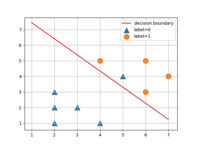
# show
#分界线也需要画出来
w0 = W[0,0]
w1 = W[1,0]
w2 = W[2,0]

plotx1 = np.arange(1, 7, 0.01)
plotx2 = -w0/w2 - (w1/w2)*plotx1
#线条画出来
plt.plot(plotx1, plotx2, c='r',label='decision boundary')

#每个点显示出来；.A表示变成array的形式
plt.scatter(xmat[:, 1][ymat==0], xmat[:, 2][ymat==0].A, marker='^', s=150, label='label=0')
plt.scatter(xmat[:, 1][ymat==1], xmat[:, 2][ymat==1].A, s=150, label='label=1')
#网格线
plt.grid()
#图标
plt.legend()
plt.show()

运行结果：

Logisic0801

step4:图的动态呈现

在之前代码的基础上进行修改

import numpy as np
import matplotlib.pyplot as plt


#def loaddata
def loaddata(filename):
    file = open(filename)
    x = []
    y = []
    for line in file.readlines():
        line = line.strip().split()
        x.append([1, float(line[0]), float(line[1])])
        y.append(float(line[-1]))
    #将列表格式变成为矩阵的格式
    xmat = np.mat(x)
    ymat = np.mat(y).T
    file.close()
    return xmat, ymat

# w calc
def w_calc(xmat, ymat, alpha= 0.001, maxIter = 10001):
    # W需要进行一个初始化看，就是里面的参数,初始化为三行一列
    W = np.mat(np.random.randn(3,1))
    #需要把每一步记录下来
    w_save = []
    # W update
    for i in range(maxIter):
        H = 1/(1+np.exp(-xmat*W))
        dw = xmat.T * (H - ymat)  #dw(3, 1)
        W -= alpha * dw
        #每100步记录一下
        if i%100 == 0:
            #如果不加copy，存的永远是最后一个数
            w_save.append([W.copy(),i])
    return W, w_save


#implement
xmat, ymat = loaddata('ytb_lr.txt')
# print('xmat:', xmat, xmat.shape)
# print('ymat:', ymat, ymat.shape)
W, w_save = w_calc(xmat, ymat, 0.001, 10000)
print('W:', W)

# show
#分界线也需要画出来

for wi in w_save:
    #如果不加clf,每一个轨迹都会保存下来，不是很好看
    plt.clf()
    #因为wi有两个数
    w0 = wi[0][0,0]
    w1 = wi[0][1,0]
    w2 = wi[0][2,0]

    plotx1 = np.arange(1, 7, 0.01)
    plotx2 = -w0/w2 - (w1/w2)*plotx1
    #线条画出来
    plt.plot(plotx1, plotx2, c='r',label='decision boundary')

    #每个点显示出来；.A表示变成array的形式
    plt.scatter(xmat[:, 1][ymat==0], xmat[:, 2][ymat==0].A, marker='^', s=150, label='label=0')
    plt.scatter(xmat[:, 1][ymat==1], xmat[:, 2][ymat==1].A, s=150, label='label=1')
    #网格线
    plt.grid()
    #图标
    plt.legend()
    #有这个命令就可以生成动画
    plt.title('iter:%s'%np.str(wi[1]))
    plt.pause(0.001)
    #如果不加show,最后执行完就会消失
plt.show()

stone

Linxia Yao

2018-08-01-逻辑回归